Basic Freeway LOS Calculator

HCM 6th Edition (2016), Chapter 12

Analyze one direction of a basic freeway segment with two or more lanes. For a highway with at-grade access, use the multilane calculator (2010 / 6th Edition).

Starting inputs are examples; replace them with site data.

Base conditions: speed and capacity adjustment factors are 1.00. This method does not model ramp junctions, weaving, queues, managed lanes, weather, or incidents.

View formulas and LOS limits

Traffic Directional hourly volume (veh/h) Lanes in one direction Peak hour factor (PHF) Total heavy vehicles (%)

Include trucks, buses and RVs. Buses and RVs count as single-unit trucks (SUTs).

Free-flow speed Speed method

Geometry Base free-flow speed (mph)

The HCM default base speed is 75.4 mph. Use a locally supported base speed when available. The resulting FFS must be 55–75 mph.

Average lane width (ft) Right-side lateral clearance (ft)

Distance from the right travel-lane edge to the nearest obstruction. Clearance of 6 ft or more has no penalty.

Total ramp density (ramps/mi)

Count on- and off-ramps in this direction within 3 mi upstream and 3 mi downstream of the segment midpoint, then divide by 6 mi. Count ramps, not interchanges. Six ramps in this window = 1 ramp/mi.

Terrain and heavy vehicles Terrain analysis

Use general terrain only when no individual grade significantly affects operation. Mountainous terrain requires a mixed-flow analysis.

Use a separately verified PCE

Verified heavy-vehicle equivalent E_T (optional) Basis / source for the PCE

A supplied PCE replaces the terrain lookup and requires its source. Clear it to resume automatic lookup.

Loads the supplied four-lane example: 2,400 veh/h, PHF 0.90, 5% heavy vehicles, base speed 60 mph, 12 ft lanes, 10 ft clearance, and 1 ramp/mi.

Calculation formulas

HCM 6th Edition basic freeway method, with SAF = CAF = 1. Keep full precision until displaying results.

1. Free-flow speed (Eq. 12-2)

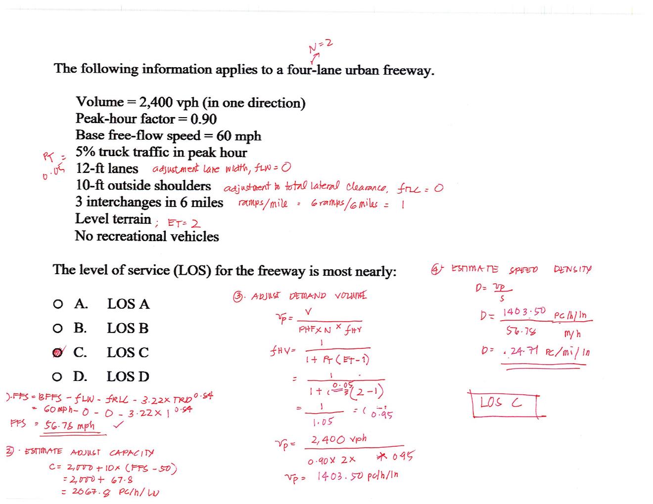
FFS = BFFS − f_LW − f_RLC − 3.22 × TRD^0.84

BFFS is base free-flow speed; TRD is ramps per mile. Use measured FFS directly when available.

Lane penalty f_LW = 0 at widths ≥12 ft, 1.9 mph for 11–<12 ft, and 6.6 mph for 10–<11 ft (Exhibit 12-20).

f_RLC = [6 − min(clearance, 6)] × k

Exhibit 12-21 is linear between clearance rows: k = 0.6, 0.4, 0.2, or 0.1 mph/ft for 2, 3, 4, or ≥5 directional lanes, respectively.

2. Heavy vehicles and flow (Eqs. 12-9, 12-10)

f_HV = 1 / [1 + P_T(E_T − 1)]
v_p = V / (PHF × N × f_HV)

P_T is the heavy-vehicle percentage divided by 100; E_T is its passenger-car equivalent (2 for level terrain, 3 for rolling terrain, or a specific-grade lookup). V is directional demand in veh/h; N is directional lanes; v_p is passenger-car flow in pc/h/ln.

3. Capacity, speed, density (Eq. 12-6, Eq. 12-1, Exhibit 12-6)

c = min[2,200 + 10(FFS − 50), 2,400]
BP = 1,000 + 40(75 − FFS)

Capacity c and speed-curve breakpoint BP are in pc/h/ln. The supported FFS range is 55–75 mph.

S = FFS, when v_p ≤ BP
S = FFS − (FFS − c/45) × [(v_p − BP)/(c − BP)]², when BP < v_p ≤ c
D = v_p / S

S is average speed in mph; D is density in pc/mi/ln. Demand above capacity is LOS F; the basic segment method does not predict speed or density in that condition.

Exhibit 12-15: density limits when demand does not exceed capacity
LOS	Density (pc/mi/ln)
A	0–11
B	>11–18
C	>18–26
D	>26–35
E	>35–45
F	Demand exceeds capacity, or density >45

Sources and edition

Supplied HCM Chapter 12 extract (Version 6.0, pp. 12-17–12-39) and the previously reviewed 6th Edition Exhibit 12-6 (p. 12-10). Specific-grade PCEs reuse the multilane calculator's verified Chapter 12 tables.

Audit and source reconciliation records corrections to the archived Python script and worked example. The example's LOS remains C with corrected arithmetic.

The supplied HCM 7th Edition reference guide is available for review. This calculator implements the verified 6th Edition base method; it does not implement the 7th Edition's connected/automated-vehicle adjustments.